Steepish Descent

Importance-weight clipping is used everywhere in machine learning. Can we get rid of it? Spoiler alert: not today.

Estimating without clipping

Several years ago, Microsoft had an online RL platform, which motivated me to work on confidence sequences for off-policy inference. These can estimate all sorts of importance-weighted quantities without explicit clipping.

Suppose you have an off-policy quantity you’d like to estimate via importance weighting, such as the (counterfactual) value of deploying a policy with parameters $\theta$,

This is a standard move where you switch to sampling from your policy $\pi$ to sampling from the policy $h$ that actually collected the data, since that is the data you actually have. However that importance weight $\pi(y|x; \theta) / h(y|x)$ can get really big, which means the naive “plugin” estimator given an empirical sample

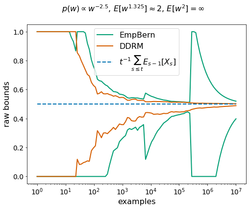
can go off the rails. So people have all sorts of hacks to keep estimators stable, such as clipping or self-normalization. Fortunately robust confidence sequences can consume unbounded importance weights with unbounded variance and adapt to an unknown finite moment greater than 1. Here’s an example from the DDRM paper with Pareto distributed importance weights.

The tl;dr is, for estimation, we can estimate the quantity of interest without explicit importance-weight clipping or other tricks. Depending upon your setting, you have a choice of techniques:

• Betting martingales: tightest, but only for evaluating a fixed policy in a stationary environment.
• Mixture of supermartingales: less tight but valid for evaluating a changing policy sequence in a nonstationary environment.
• DDRM: a more complex mixture of supermartingales designed for extreme robustness.

By the way you can estimate other functionals besides the mean. In the csrobust repository there are examples of covering the entire (counterfactual) CDF.

Learning without Clipping?

If we can estimate without (explicitly) clipping, and if learning is optimization of an estimator, then can we learn without clipping? It feels like the answer is yes.

But what would this look like? In the confidence sequences above, you don’t actually get a point estimate. Instead you get a lower bound estimate that converges to the true value from below, and an upper bound estimate that converges to the true value from above. Optimizing a lower bound corresponds to a pessimistic learning strategy, whereas optimizing an upper bound corresponds to an optimistic strategy. Optimizing an upper bound might induce beneficial exploration if the optimized policy is used to collect more data, but if the data is exogenous it could be dangerous. Optimizing a lower bound is safe but conservative, so I started there.

Lower bound optimization

The simplest lower bound is derived from a betting martingale, which technically only applies in stationary environments where the policy being evaluated is not changing. Fortunately betting martingales are valid under a changing logging policy sequence, and so are a good match to batch policy gradient in modern RL setups with asynchronous updates, where the rollout workers are using older parameters than the training worker, if we make a fresh lower bound for each batch.

Suppose our dataset consists only of non-negative rewards $\{ r_t(\theta) \}$, and the reward depends upon our optimization parameter $\theta$. For now $\theta$ is considered fixed. A betting martingale is driven by a wealth process

Here $b \in [0,1)^T$ is an adapted betting process, meaning each $b_t$ has to be chosen before seeing $r_t(\theta)$. Assuming $r_t(\theta)$ each have the same mean $v$, then $W(v,b)$ is a non-negative martingale and unlikely to ever get large, therefore using Ville’s inequality, we can reject values of $z$ where $W$ is large. The wealth level for rejection with confidence $\alpha$ would be $-\log(\alpha)$. However to evaluate this we have to choose an adapted betting sequence, and it is a standard move to pretend to run a no-regret algorithm, plug in the regret bound, and then simply compare with the best fixed bet in hindsight. If we use Cover’s universal portfolio we can compare with the best bet in hindsight, in exchange for a larger wealth threshold $\log\left(\frac{1+T}{\alpha}\right)$. So that leads to the following optimization problem to define a lower bound

Assuming at least one reward is non-zero, we have a non-trivial lower bound $v^*(\theta)$ and we can use the envelope theorem to take the gradient of it

It’s not obvious but the above is typically a convex combination of individual gradients, unless the observed rewards have tiny variance, in which case it is a slightly sub-convex combination with a worst case slack of circa $\log(T)/T.$

We can specialize this to an importance-weighted reward. Now the dataset consists of $\{ (x_t, y_t, h_t, r_t) \}$ where $x_t$ is a prompt, $y_t$ is a completion, $h_t$ is the policy that generated the datapoint, and $r_t$ is a scalar. Furthermore we are evaluating$\pi(y_t | x_t; \theta).$ Then

This looks like a self-normalizing estimator, which is numerically stable even when a single importance weight gets huge. However, when a single importance gets huge, it dominates the gradient: the effective sample size goes to 1. In particular if the large importance weight sample has small but non-zero reward, it can dominate the gradient of a small importance weight sample that has a larger reward. This is not what you want from a gradient in RL: in real life large rewards are rare and when you find them you want to move towards them aggressively.

So for extreme importance weight robustness in off-policy RL, betting martingales are apparently “not it”. But perhaps one of the more sophisticated mixture martingales would work.